Your Estimate Is a Dot. Here's the Shape It's Hiding.
PERT gives you a number. Monte Carlo gives you the probability you'll actually hit it. A worked example showing why the difference matters.
Your project manager says the project will take 51 days. You commit to the client. On day 44, the team ships. You look like a hero — but only by accident. The estimate was wrong by a week. It just happened to be wrong in the comfortable direction.
Next time, it won’t be.
The problem isn’t bad estimators. The problem is that a single number — even a mathematically sound one — hides the shape of the risk underneath it.
The Point Estimate Trap
PERT (Programme Evaluation and Review Technique) is the standard. You collect three estimates per task — optimistic, most likely, pessimistic — and compute an expected duration. It’s been the textbook method since the 1950s, and for good reason: it forces estimators to think about uncertainty rather than pretending a single guess is precise.
But PERT has a structural blind spot. When tasks run in parallel, PERT sums the expected values along the longest path. That sounds reasonable until you realise: the longest path changes depending on which tasks run long.
Consider a simple dependency network:
Requirements → Design → Backend  ─┐
                     → Frontend ─┤→ Integration → Testing
Backend and Frontend run in parallel after Design. PERT picks the longer expected path (Backend) and sums along it. But in reality, sometimes Frontend runs long and becomes the critical path. PERT can’t see that. It gives you one path, one number, one false certainty.
For this 6-task project, PERT’s naive sum produces 51.5 days.
Monte Carlo produces a mean of 41.1 days.
That’s a 10-day gap — not because someone estimated badly, but because PERT double-counts duration on parallel paths. Those 10 days are phantom padding that doesn’t correspond to any real work.
What Monte Carlo Actually Does
The idea is simple: instead of calculating one answer, simulate the project thousands of times.
Each simulation draws a random duration for every task from its probability distribution (the same three-point estimates PERT uses). It respects the dependency network — Integration can’t start until both Backend and Frontend finish. It records the total project duration.
After 10,000 simulations, you don’t have a number. You have a distribution. And that distribution answers a fundamentally different question.
PERT answers: “How long will it take?”
Monte Carlo answers: “What’s the probability we finish by Thursday?"
"Can We Ship in 45 Days?”
Here’s the same 6-task project, simulated 10,000 times:
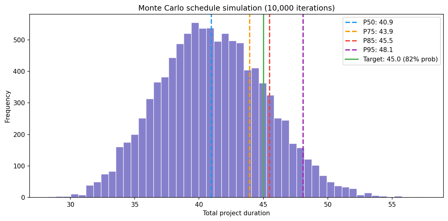
The histogram shows every possible outcome. The green line is your stakeholder’s question: 45 days.
The answer: 82% likely.
Not great, not terrible. But now you can have an honest conversation. “We have an 82% chance of hitting your date. If you need 95% confidence, we need 48 days. If you’re comfortable with a coin flip plus a bit, 41 days is the median.”
Those vertical lines are commitment levels:
| Percentile | Days | What It Means |
|---|---|---|
| P50 | 40.9 | Coin flip — half the simulations finish later |
| P75 | 43.9 | Reasonable confidence, some residual risk |
| P85 | 45.5 | Recommended commitment — balances confidence against padding |
| P95 | 48.1 | Conservative buffer — only 1 in 20 simulations runs longer |
P85 is the sweet spot. It’s confident enough to commit to, honest enough to not waste resources on phantom buffer.
The PERT Phantom
Now consider what happens if you commit to PERT’s estimate of 51.5 days instead.
Every single simulation — all 10,000 of them — finishes before that date. The probability of hitting 51.5 days is 100%. You’ve committed to a target that is impossible to miss.
That sounds safe. It’s actually wasteful. P85 gives you 45.5 days at high confidence. The remaining 6 days are phantom duration — structural padding from PERT’s inability to handle parallel paths, not a deliberate buffer.
In a competitive bid, this is the difference between winning and losing. In an internal context, it’s the difference between shipping in Q2 and slipping to Q3 “just to be safe.” The phantom comes from PERT’s structural limitation: it sums expected values along a single critical path, but the critical path isn’t fixed.
The Path That Shifts
This is the second insight Monte Carlo provides that PERT cannot.
Deterministic critical path analysis gives you one path: Requirements → Design → Backend → Integration → Testing. Backend is critical. Frontend is not. Simple.
Monte Carlo tells you that’s only true 85% of the time.
In the other 15% of simulations, Frontend runs long enough to become the bottleneck. Integration waits for Frontend, not Backend. The critical path shifts.
| Task | Critical Path Frequency |
|---|---|
| Requirements | 100% |
| Design | 100% |
| Backend | 85.4% |
| Frontend | 14.6% |
| Integration | 100% |
| Testing | 100% |
A task that’s critical in 15% of simulations is a risk that deterministic analysis literally cannot see. If your Frontend lead goes on leave and nobody flags it — because Frontend “isn’t on the critical path” — you’ve got a one-in-seven chance of a surprise delay.
Monte Carlo makes that visible.
When to Use Which
Not every project needs a full simulation. Here’s the decision boundary:
PERT is sufficient when:
- Tasks are sequential (no parallel paths)
- The critical path is obvious and stable
- You need a sanity check, not a commitment
Monte Carlo earns its keep when:
- Parallel paths exist — the critical path can shift between simulations
- A stakeholder is asking for a confidence level, not just an estimate
- You’re making a contractual or financial commitment based on the timeline
- Estimates are skewed (optimistic ≠ pessimistic spread) — the distribution shape matters
The key insight: when there are no parallel paths, Monte Carlo and PERT agree on the mean. Monte Carlo’s value in that case is the distribution itself — you still get P85 and P95, which PERT’s Gaussian approximation can only guess at.
Try It
The Monte Carlo module is open source, available as both a Python library and
a REST API. It’s designed to be spun up locally with uv — clone the repo
and you’re running in minutes. Write a few lines of Python or hit the FastAPI
endpoints with JSON; data is stored in local SQLite. MIT-licensed, so you can
embed it in existing commercial products.
- Python:
from app.montecarlo.core import simulate_schedule - API:
POST /montecarlo/simulate— stateless simulation from task list - API:
POST /montecarlo/scenarios— save and compare scenarios over time
Source: github.com/lemur47/logic
Your estimate is a dot. The distribution is the truth. The question isn’t “how long will it take?” — it’s “how confident are we, and what are we willing to pay for more confidence?”
This post is part of the Cognition as Code series — encoding PMO decision-making as executable logic. The Monte Carlo module was built, tested, and verified in Sprint 6 alongside PERT, EVM, Bayesian, and TCO modules.